Zeeman effect

The Zeeman effect ( /ˈzeɪmən/; IPA: [ˈzeːmɑn]) is the splitting of a spectral line into several components in the presence of a static magnetic field. It is analogous to the Stark effect, the splitting of a spectral line into several components in the presence of an electric field. The Zeeman effect is very important in applications such as nuclear magnetic resonance spectroscopy, electron spin resonance spectroscopy, magnetic resonance imaging (MRI) and Mössbauer spectroscopy. It may also be utilized to improve accuracy in Atomic absorption spectroscopy.

When the spectral lines are absorption lines, the effect is called Inverse Zeeman effect.

The Zeeman effect is named after the Dutch physicist Pieter Zeeman.

1 Introduction
2 Theoretical presentation
3 Weak field (Zeeman effect)
- 3.1 Example: Lyman alpha transition in hydrogen
4 Strong field (Paschen-Back effect)
5 See also
6 References
- 6.1 Historical
- 6.2 Modern

Introduction

In most atoms, there exist several electron configurations with the same energy, so that transitions between these configurations and another correspond to a single spectral line. The presence of a magnetic field breaks this degeneracy, since the magnetic field interacts differently with electrons with different quantum numbers, slightly modifying their energies. The result is that, where there were several configurations with the same energy, they now have different energies, giving rise to several very close spectral lines.

Without a magnetic field, configurations a, b and c have the same energy, as do d, e and f. The presence of a magnetic field (B) splits the energy levels. Therefore, a line produced by a transition from a, b or c to d, e or f will now be split into several components between different combinations of a, b, c and d, e, f. However, not all transitions will be possible (in the dipole approximation), as governed by the selection rules.

Since the distance between the Zeeman sub-levels is proportional to the magnetic field, this effect can be used by astronomers to measure the magnetic field of the Sun and other stars.

There is also an anomalous Zeeman effect that appears on transitions where the net spin of the electrons is not 0, the number of Zeeman sub-levels being even instead of odd if there's an uneven number of electrons involved. It was called "anomalous" because the electron spin had not yet been discovered, and so there was no good explanation for it at the time that Zeeman observed the effect.

At higher magnetic fields the effect ceases to be linear. At even higher field strength, when the strength of the external field is comparable to the strength of the atom's internal field, electron coupling is disturbed and the spectral lines rearrange. This is called the Paschen-Back effect.

Theoretical presentation

The total Hamiltonian of an atom in a magnetic field is

$H = H_0 %2B V_M,\$

where $H_0$ is the unperturbed Hamiltonian of the atom, and $V_M$ is perturbation due to the magnetic field:

$V_M = -\vec{\mu} \cdot \vec{B},$

where $\vec{\mu}$ is the magnetic moment of the atom. The magnetic moment consists of the electronic and nuclear parts, however, the latter is many orders of magnitude smaller and will be neglected further on. Therefore,

$\vec{\mu} = -\mu_B g \vec{J}/\hbar,$

where $\mu_B$ is the Bohr magneton, $\vec{J}$ is the total electronic angular momentum, and $g$ is the g-factor. The operator of the magnetic moment of an electron is a sum of the contributions of the orbital angular momentum $\vec L$ and the spin angular momentum $\vec S$ , with each multiplied by the appropriate gyromagnetic ratio:

$\vec{\mu} = -\mu_B (g_l \vec{L} %2B g_s \vec{S})/\hbar,$

where $g_l = 1$ and $g_s \approx 2.0023192$ (the latter is called the anomalous gyromagnetic ratio; the deviation of the value from 2 is due to Quantum Electrodynamics effects). In the case of the LS coupling, one can sum over all electrons in the atom:

$g \vec{J} = \left\langle\sum_i (g_l \vec{l_i} %2B g_s \vec{s_i})\right\rangle = \left\langle (g_l\vec{L} %2B g_s \vec{S})\right\rangle,$

where $\vec{L}$ and $\vec{S}$ are the total orbital momentum and spin of the atom, and averaging is done over a state with a given value of the total angular momentum.

If the interaction term $V_M$ is small (less than the fine structure), it can be treated as a perturbation; this is the Zeeman effect proper. In the Paschen-Back effect, described below, $V_M$ exceeds the LS coupling significantly (but is still small compared to $H_{0}$ ). In ultrastrong magnetic fields, the magnetic-field interaction may exceed $H_0$ , in which case the atom can no longer exist in its normal meaning, and one talks about Landau levels instead. There are, of course, intermediate cases which are more complex than these limit cases.

Weak field (Zeeman effect)

If the spin-orbit interaction dominates over the effect of the external magnetic field, $\scriptstyle \vec L$ and $\scriptstyle \vec S$ are not separately conserved, only the total angular momentum $\scriptstyle \vec J = \vec L %2B \vec S$ is. The spin and orbital angular momentum vectors can be thought of as precessing about the (fixed) total angular momentum vector $\scriptstyle \vec J$ . The (time-)"averaged" spin vector is then the projection of the spin onto the direction of $\scriptstyle \vec J$ :

$\vec S_{avg} = \frac{(\vec S \cdot \vec J)}{J^2} \vec J$

and for the (time-)"averaged" orbital vector:

$\vec L_{avg} = \frac{(\vec L \cdot \vec J)}{J^2} \vec J.$

Thus,

$\langle V_M \rangle = \frac{\mu_B}{\hbar} \vec J(g_L\frac{\vec L \cdot \vec J}{J^2} %2B g_S\frac{\vec S \cdot \vec J}{J^2}) \cdot \vec B.$

Using $\scriptstyle \vec L = \vec J - \vec S$ and squaring both sides, we get

$\vec S \cdot \vec J = \frac{1}{2}(J^2 %2B S^2 - L^2) = \frac{\hbar^2}{2}[j(j%2B1) - l(l%2B1) %2B s(s%2B1)],$

and: using $\scriptstyle \vec S = \vec J - \vec L$ and squaring both sides, we get

$\vec L \cdot \vec J = \frac{1}{2}(J^2 - S^2 %2B L^2) = \frac{\hbar^2}{2}[j(j%2B1) %2B l(l%2B1) - s(s%2B1)].$

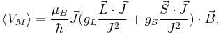
Combining everything and taking $\scriptstyle J_z = \hbar m_j$ , we obtain the magnetic potential energy of the atom in the applied external magnetic field,

$\begin{align} V_M &= \mu_B B m_j \left[ g_L\frac{j(j%2B1) %2B l(l%2B1) - s(s%2B1)}{2j(j%2B1)} %2B g_S\frac{j(j%2B1) - l(l%2B1) %2B s(s%2B1)}{2j(j%2B1)} \right]\\ &= \mu_B B m_j \left[1 %2B (g_S-1)\frac{j(j%2B1) - l(l%2B1) %2B s(s%2B1)}{2j(j%2B1)} \right], \\ &= \mu_B B m_j g_j \end{align}$

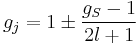
where the quantity in square brackets is the Lande g-factor g_J of the atom ( $g_L = 1$ and $\scriptstyle g_S \approx 2$ ) and $m_j$ is the z-component of the total angular momentum. For a single electron above filled shells $s = 1/2$ and $j = l \pm s$ , the Lande g-factor can be simplified into:

$g_j = 1 \pm \frac{g_S-1}{2l%2B1}$

Example: Lyman alpha transition in hydrogen

The Lyman alpha transition in hydrogen in the presence of the spin-orbit interaction involves the transitions

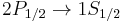$2P_{1/2} \to 1S_{1/2}$ and $2P_{3/2} \to 1S_{1/2}.$

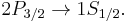
In the presence of an external magnetic field, the weak-field Zeeman effect splits the 1S_1/2 and 2P_1/2 states into 2 levels each ( $m_j = 1/2, -1/2$ ) and the 2P_3/2 state into 4 levels ( $m_j = 3/2, 1/2, -1/2, -3/2$ ). The Lande g-factors for the three levels are:

$g_J = 2$ for $1S_{1/2}$ (j=1/2, l=0)

$g_J = 2/3$ for $2P_{1/2}$ (j=1/2, l=1)

$g_J = 4/3$ for $2P_{3/2}$ (j=3/2, l=1).

Note in particular that the size of the energy splitting is different for the different orbitals, because the g_J values are different. On the left, fine structure splitting is depicted. This splitting occurs even in the absence of a magnetic field, as it is due to spin-orbit coupling. Depicted on the right is the additional Zeeman splitting, which occurs in the presence of magnetic fields.

Strong field (Paschen-Back effect)

The Paschen-Back effect is the splitting of atomic energy levels in the presence of a strong magnetic field. This occurs when an external magnetic field is sufficiently large to disrupt the coupling between orbital ( $\vec L$ ) and spin ( $\vec S$ ) angular momenta. This effect is the strong-field limit of the Zeeman effect. When $s = 0$ , the two effects are equivalent. The effect was named after the German physicists Friedrich Paschen and Ernst E. A. Back.

When the magnetic-field perturbation significantly exceeds the spin-orbit interaction, one can safely assume $[H_{0}, S] = 0$ . This allows the expectation values of $L_{z}$ and $S_{z}$ to be easily evaluated for a state $|A\rangle$ :

$\langle A| \left( H_{0} %2B \frac{B_{z}\mu_B}{\hbar}(L_{z}%2Bg_{s}S_z) \right) |A \rangle = E_{0} %2B B_z\mu_B (m_l %2B g_{s}m_s).$

The above may be read as implying that the LS-coupling is completely broken by the external field. The $m_l$ and $m_s$ are still "good" quantum numbers. Together with the selection rules for an electric dipole transition, i.e., $\Delta s = 0, \Delta m_s = 0, \Delta l = \pm 1, \Delta m_l = 0, \pm 1$ this allows to ignore the spin degree of freedom altogether. As a result, only three spectral lines will be visible, corresponding to the $\Delta m_l = 0, \pm 1$ selection rule. The splitting $\Delta E = B \mu_B \Delta m_l$ is independent of the unperturbed energies and electronic configurations of the levels being considered. It should be noted that in general (if $s \ne 0$ ), these three components are actually groups of several transitions each, due to the residual spin-orbit coupling.

References

Historical

Condon, E. U.; G. H. Shortley (1935). The Theory of Atomic Spectra. Cambridge University Press. ISBN 0-521-09209-4. (Chapter 16 provides a comprehensive treatment, as of 1935.)
Zeeman, P. (1897). "On the influence of Magnetism on the Nature of the Light emitted by a Substance". Phil. Mag. 43: 226.
Zeeman, P. (1897). "Doubles and triplets in the spectrum produced by external magnetic forces". Phil. Mag. 44: 55.
Zeeman, P. (11 February 1897). "The Effect of Magnetisation on the Nature of Light Emitted by a Substance". Nature 55 (1424): 347. Bibcode 1897Natur..55..347Z. doi:10.1038/055347a0. http://www.nature.com/nature/journal/v55/n1424/abs/055347a0.html.

Modern

Feynman, Richard P., Leighton, Robert B., Sands, Matthew (1965). The Feynman Lectures on Physics, Vol. 3. Addison-Wesley. ISBN 0-201-02115-3.
Forman, Paul (1970). "Alfred Landé and the anomalous Zeeman Effect, 1919-1921". Historical Studies in the Physical Sciences 2: 153–261.
Griffiths, David J. (2004). Introduction to Quantum Mechanics (2nd ed.). Prentice_Hall!Prentice Hall. ISBN 0-13-805326-X.
Liboff, Richard L. (2002). Introductory Quantum Mechanics. Addison-Wesley. ISBN 0-8053-8714-5.
Sobelman, Igor I. (2006). Theory of Atomic Spectra. Alpha Science. ISBN 1-84265-203-6.
Foot, C. J. (2005). Atomic Physics. ISBN 0198506961.